Showing posts with label neuroscience. Show all posts

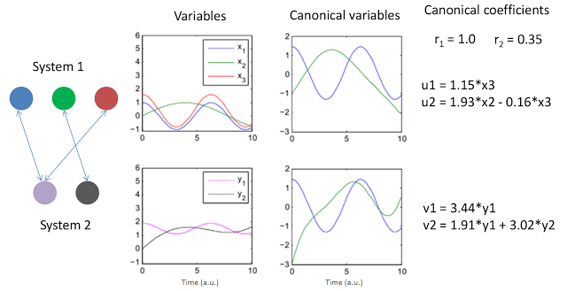
Canonical correlation analysis (CCA) is a tool to find relations among two sets of random variables. The result of CCA is a new pair of sets of random variables, the canonical variables, which represent potential linear relations between the original sets. As a tool to analyze the relation between two signals or time domain systems, CCA is a powerful method to discover intrinsic linear relations between the two systems.

A few days ago I had to understand how CCA works for a presentation and found relatively little information online, and almost no simple examples that I could use to visualize it. At the end it resulted to be a rather simple concept. Here I present a simple example with artificial signals I designed for my presentation.

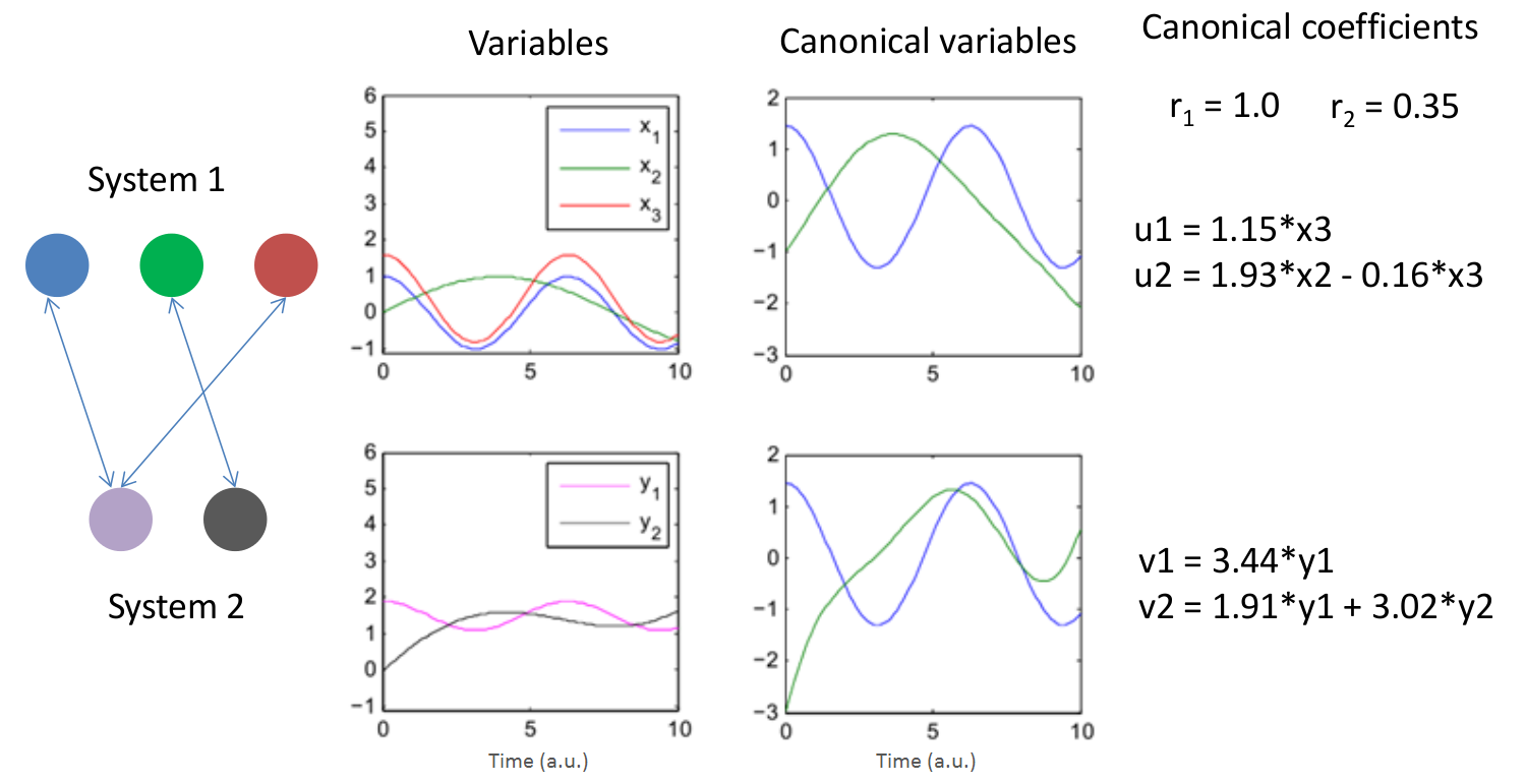
The above figure presents two simple systems and the resulting canonical variables and coefficients. The signals were conveniently created to display simple linear relations. Note that x1 and x3 are basically just a scaled version of y1 so one would expect a high correlation among them and potentially a canonical variable would explain that. The variables x2 and y2 also exhibit a relation but this time a rather weak one. The graph to the left represents this relationships with arrows. Note that CCA allows to compare sets with different numbers of variables, just another beauty of the method.

The results of CCA for this example are shown no the right of the above figure. The two canonical coefficients show the "strength" of the relations between the two sets (the method produces two i.e. the minimum between the number of elements of the two sets: 2 vs 3). The two pairs of canonical "systems": (u1, u2) and (v1, v2) represent the linear combinations of variables of each system in the form they produce the strongest correlations among the original sets (x's and y's). As such they can be written as linear equations from the original variables.

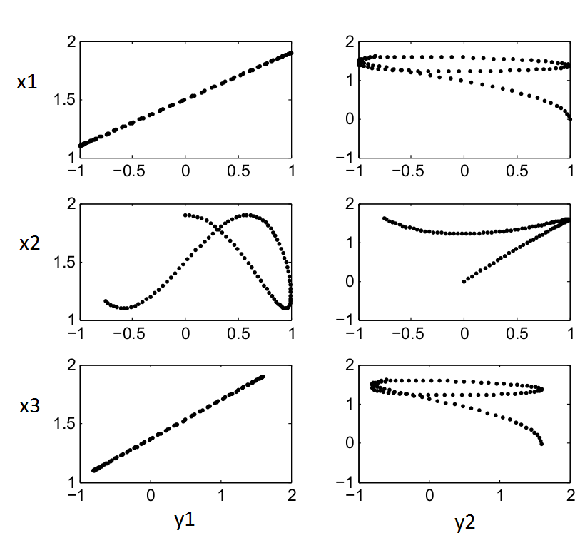
The Matlab code below was used to produce the figures above. Another for to visualize the relations between the variables is to plot all possible combinations of variables as scatter plots (x's vs y's). That plot is shown after the code.

%% Create example canonical correlation plots in Matlab

% Build some simple signals with optional noise (s)
t = 0:0.1:10;
l = length(t);
s = 0;
X(:,1) = cos(t) + s*rand(1,l);
X(:,2) = sin(t/2.5) + s*rand(1,l);
X(:,3) = 1.2*cos(t) + 0.4 + s*rand(1,l) + t*0.0;

Y(:,1) = 0.4*cos(t) + 1.5 + s*rand(1,l);
Y(:,2) = sin(t/2.2+0.4) - 0.4 + t*0.3 + s*rand(1,l);

% Plot signals over time
figure(1)
subplot(2,2,1); plot(t,X); ylim([-1.1 6])
legend('x_1','x_2','x_3')
subplot(2,2,3); plot(t,Y(:,1),'m',t,Y(:,2),'k'); ylim([-1.1 6])
legend('y_1','y_2')

% It is usually prudent to check the rank, just display it
rank(X)
rank(Y)

% Perform CCA using Matlabs function
[A,B,r,U,V] = canoncorr(X,Y);

% Just print out results
A,B,r

subplot(2,2,2); plot(t,U); ylim([-3 2])
subplot(2,2,4); plot(t,V); ylim([-3 2])

%% Plot canonical variables 
figure(2); clf; 
subplot(2,1,1); hold all; plot(t,X*A); plot(t,U);
subplot(2,1,2); hold all; plot(t,Y*B); plot(t,V);

%% Plot signals against each other
figure(3)
subplot(3,2,1); plot(X(:,1),Y(:,1),'k.')
subplot(3,2,3); plot(X(:,2),Y(:,1),'k.')
subplot(3,2,5); plot(X(:,3),Y(:,1),'k.')
subplot(3,2,2); plot(X(:,1),Y(:,2),'k.')
subplot(3,2,4); plot(X(:,2),Y(:,2),'k.')
subplot(3,2,6); plot(X(:,3),Y(:,2),'k.')

% Some information about their correlations
p = corrcoef([X Y]);
p = p(1:3,4:5)

The scatter plot for figure(3):

This is a simple compilation and a taxonomy attempt of Python plotting libraries. This is focused on web alternatives that can be combined with iPython Notebook but at least one is desktop based. I used Python for most of my dissertation writing and now, during my Postdoc, the time to produce pretty publication plots is near. The list adds some details of the project as reported by its GitHub repo. This builds upon Nathan Lemoine's post.
Maplotlib and Matplotlib improvements:

Matplotlib: 14,758 commits, 4 branches, 43 releases, 360 contributors, Jul 12, 2015
Holoviews: 3,860 commits, 4 branches, 10 releases, 9 contributors, Jul 11, 2015
Seaborn: 1,378 commits, 10 branches, 9 releases, 38 contributors, Jul 10, 2015
ggplot: 731 commits, 3 branches, 0 releases, 40 contributors, Jun 11, 2015
mpld3: 540 commits, 13 branches, 1 releases, 27 contributors, Jul 6, 2015
Prettyplotlib: 252 commits, 5 branches, 0 releases, 21 contributors, Oct 6, 2014

Alternatives independent of Matplotlib based on d3:

plot.ly: 1,215 commits 26 branches 4 releases 8 contributors Jul 10, 2015
Vincent: 419 commits, 2 branches, 8 releases, 23 contributors, Jan 28, 2015
d3py: 161 commits, 3 branches, 0 releases, 8 contributors, Feb 7, 2014

Alternatives independent of Matplotlib:

Bokeh: 9,161 commits, 29 branches, 51 releases, 98 contributors, Jul 10, 2015
Veusz: 2,615 commits, 13 branches, 39 releases, 14 contributors, Jul 11, 2015
Python-highchart: 139 commits, 3 branches, 13 releases, 4 contributors, Jul 6, 2015

Image: Bokeh


Some facts about brain density:

  • The size of a bee's  brain is around 1 cubic millimeter and contains around 1 million neurons (C. B. Don). This is enough to perform all basic movement activities, communication, and even a social life. The human brain is around 1.2x10⁶ cubic millimeters.
  • “One cubic millimeter of cerebral cortex contains roughly 50,000 neurons, each of which establishes approximately 6,000 synapses with neighboring cells (Beaulieu and Colonnier, 1983). These 300,000,000 interconnections are highly specific: neurons innervate some target cells but avoid others. Of course, a cubic millimeter is but a miniscule part of the full circuitry, which is estimated to contain 60x1012” (CRL Harvard).
  • “One cubic millimeter is 1/1000 of a cubic centimeter and 1/1000000 (10-6) of the entire volume of the brain. We can scale the total number of connections in the brain (using the high estimate of 1015 connections in the brain) then we find that there are 109 connections in a cubic millimeter of the brain.” The Astronomist
  • Another estimate of connectivity density: “In every cubic millimeter of cortical tissue about a million of neurons must be wired appropriately for their respective functions such as the analysis of sensory inputs, the storage of skills and memory, or for motor control.” Max-Planck-Institute for Dynamics and Self-Organization
  • One cubic millimeter of cortical tissue amounts to 4 km of axon cables, 500 m of dendrites and around one billion synapses (Braitenberg and Schüz, 1998).
  • “Imaging a cubic millimeter of brain tissue requires one petabyte of storage space (106 gigabytes = 1000 terabytes = 1 petabyte)!  With the current technology, it would take about 10 million years to map every synapse in a human brain, and would require several million more petabytes of data to store the information.” Knowing Neurons
Image: Hippocampus Brainbow by Dr. Tamily Weissman

Note: This post is an update from an older post in September 2007, created after a quote from the Max-Planck-Institute for Dynamics and Self-Organization in Germany. In 2008 I joined this institute to write my doctoral dissertation.

These guys at Georgia tech connected a brain culture with real cells to a flight simulator and were able to control the roll and pitch of an F22.

Old article but still amazing:

New Scientist article.

YouTube video.

Original video was here: http://www.youtube.com/v/0jeV77dSyMI

Update (6.4.15): This history was quite a life changer for me. Quite cool and amazing job that partially got me into neuroscience. In retrospective not great science but quite catchy, and on the time, an eye opener of how advanced neuroscience was by 2004.

Photo: Lockheed Martin F-22A Raptor fighter streaks by the ramp at the 2008 Joint Services Open House (JSOH) airshow at Andrews AFB by Rob Shenk from Great Falls, VA, USA.